
Small hydro plant design tutorial 3/3: sections, draft tube and balancing
The draft tube, or diffuser, recovers the velocity left behind the runner by turning it into suction at its outlet; balancing then adjusts the runner so that gross head, head losses and absorbed head close up, and cavitation is judged last. This third part of the hydroelectric plant tutorial completes the 12 m³/s site under 4 m: draft tube, Bernoulli balance of the flow path, solver, cavitation, results, and the study files to download.
Hydroelectric turbines chapter:
- Power capture with a Kaplan turbine 1/3: the components and how they work
- Power capture with a Kaplan turbine 2/3: the distributor-runner relationship
- Power capture with a Kaplan turbine 3/3: the design method
- Hydroelectric plant tutorial 1/3: site power and runner
- Hydroelectric plant tutorial 2/3: distributor and spiral casing
- Hydroelectric plant tutorial 3/3: draft tube, balancing and cavitation
Contents of this page:
- Choosing the sections: velocity, flow rate and head losses
- The draft tube: outlet section, cone and pressure recovery
- The Bernoulli balance of the flow path and the piezometric graph
- Balancing the runner with the solver
- Cavitation: runner height and rotational speed
- The results, the project and the kit
- For the record: the manual method
1: Choosing the sections: velocity, flow rate and head losses
Two basic rules guide the choice of sections: minimize head losses, which enlarges, and concentrate the energy in the precious components, which reduces. For an incompressible fluid, the flow rate is the same at every point of the flow path, and the velocity at each section is Q/S: controlling the sections is controlling the velocities, hence the losses.
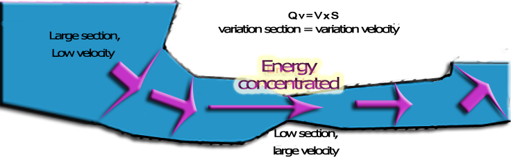
Large supply sections, concentrated technical zone, gradual transitions.
The supply zone: sections as wide as possible, up to the spiral casing.
On the example, the water goes from 2.45 m/s in the pipe to 1.77 m/s in the spiral casing, 4.10 m/s at the guide vane passage, 5.26 m/s in the runner, 4.38 m/s at the draft tube inlet and 2 m/s at its outlet. Heliciel displays each of these velocities, with the pressure and the section, in the vertical view and the piezometric graph.
2: The draft tube: outlet section, cone and pressure recovery
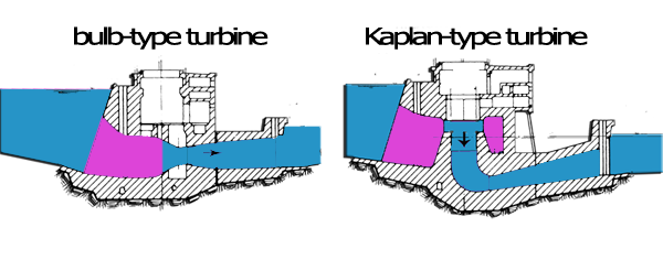
The runner cannot take all the kinetic energy of the water: some remains behind it, and in the downstream reservoir, which is large, we can enlarge the section down to a very low velocity. A diverging cone, the draft tube, makes this transition. By Bernoulli, slowing the water from its outlet towards the reservoir creates a suction at the runner outlet: the runner sees a head larger than its mere height above the tailwater. If the cone opens too fast, turbulence eats up the gain: the optimum angle is about 6°, and for compactness 12 to 14° are accepted.
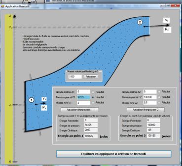
The suction at the runner outlet, created by the deceleration in the draft tube.
In the Vacuum duct tab, the AutoSize button sets the outlet section for 2 m/s at maximum flow and the length for a 14° cone: rectangular outlet of 6 m², length 3.65 m, half-angle 7°. Heliciel computes the suction gain (V²inlet − V²outlet)/2g = 0.77 m, and the losses: cone 0.067 m, friction 0.009 m, outlet kinetic energy 0.204 m, total 0.28 m. The elbow that brings the draft tube back to horizontal costs a further 0.22 m.
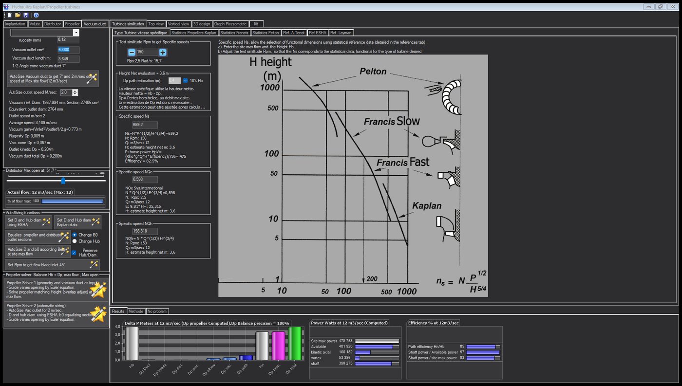
The draft tube of the example, sized for a 2 m/s outlet.
Hydro Turbine interface of Heliciel (requires a Mecaflux Suite license)
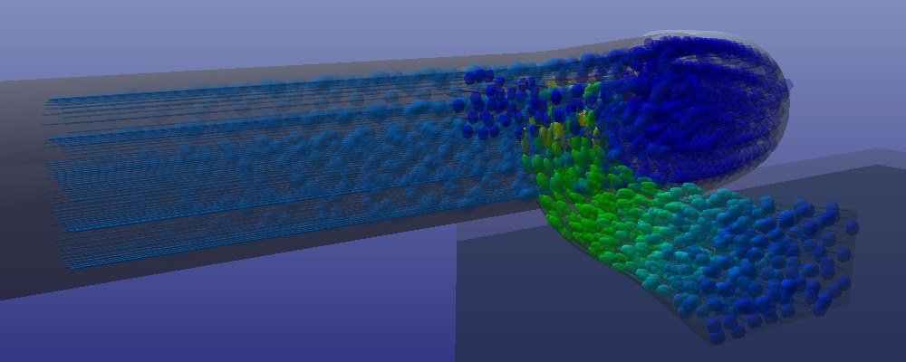
The elbow draft tube with its rectangular outlet, seen from downstream: the trajectories slow down and spread out to the river.
3: The Bernoulli balance of the flow path and the piezometric graph
Heliciel follows the energy of the water at ten points, from the upstream reservoir to the tailwater, applying Bernoulli from point to point: pressure, velocity, elevation, and the head loss of each stretch. At the runner inlet, the velocity includes its tangential component, the swirl given by the distributor: the static pressure there is lower by as much. The vertical view displays these values on the dimensioned drawing, the piezometric graph plots them.
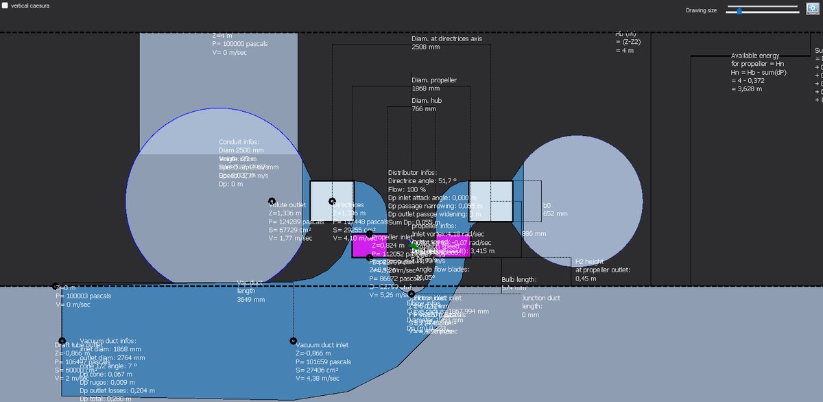
The dimensioned vertical view: pressure, velocity and section at each point of the flow path.
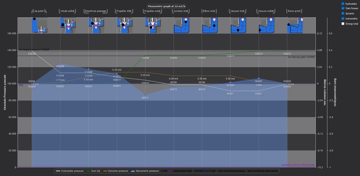
The piezometric graph: the pressure drops at the runner outlet, 86.7 kPa, and recovers in the draft tube up to the reservoir.
The sum of the losses along the path is 0.585 m: pipe 0.027, distributor 0.055, elbow 0.223, draft tube 0.280. The net head is therefore 3.415 m, 85 % of the gross head, and it is what the runner must absorb.
4: Balancing the runner with the solver
The Propeller Solver 2 does it all in one go: draft tube at 2 m/s, runner by ESHA, b0 by equalization, then balancing. It opens the guide vanes by Euler's equation and adjusts the blade overlap, by a repeated runner calculation, until the absorbed head equals the net head. Two minutes later, its message says:
"Propeller Dp (3,415 = static 2,961 + swirl 0,453) + Flow path Dp (0,585) = 4,000 m at the flow 12 m3/sec and overlap −17,9 % are balanced on the site Height 4 m, with a Delta precision of 5 pascals. Result precision = 100 %"
Let us read it. The runner absorbs 3.415 m: 2.961 m of static pressure head, and 0.453 m of swirl head, the rotation that the distributor had taken from the head and that the runner converts into torque. With the 0.585 m of losses, the total is 4.000 m: the gross head, to within 5 Pa. The chord overlap settled at −17.9 %. The runner delivers 390 kW at the shaft, for an axial thrust of 66 kN on the thrust bearing and a torque of 24.8 kN·m.
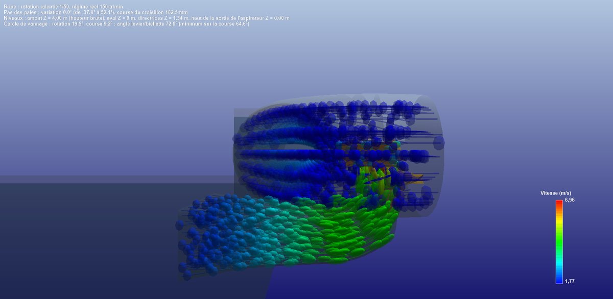
The dimensioned vertical cut, in three-quarter view: the 2,508 mm guide vane axis circle, the 1,868 mm runner, the 766 mm hub, b0, the bulb, the 3,649 mm draft tube, H2 and the 4 m gross head.
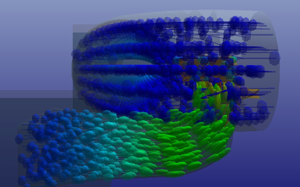
The front cut: the particles swirl in the casing, dive through the runner and slow down in the elbow draft tube.
5: Cavitation: runner height and rotational speed
After balancing, Heliciel judges cavitation: on the flow path, at each point, and on the blades, judged at the runner outlet pressure, 86.7 kPa here. The verdict is only information: nothing is corrected by itself, and it is up to us to act. Two levers are in our hands, and we tried them one after the other.
- The runner height. At 230 rpm and H2 = 1.5 m, four blade elements out of five cavitated, the runner outlet pressure falling to 69 kPa. Lowering the runner to 0.45 m above the tailwater, the minimum the bulb allows, the outlet pressure rose back to 79 kPa and three elements still cavitated.
- The rotational speed. Going from 230 to 150 rpm, the runner proposed by ESHA grows from 1,574 to 1,868 mm, goes from three to five blades, and the velocities drop. Only one element out of five remains flagged, at the blade tip; the flow path is sound.
This last element is the design margin still to be taken: an even lower speed, a larger runner, or a finer study of the blade tip. We leave this point open, as a preliminary design would.
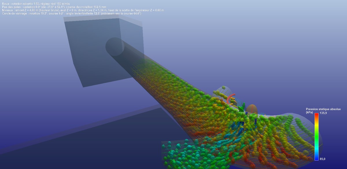
The three-quarter cut, trajectories coloured by pressure: the pressure drops from the casing to the runner, then recovers in the draft tube.
6: The results, the project and the kit
The Results tab sums up the balance in three charts. The heads: each loss, the net head, the runner head and the total. The powers: 471 kW gross, 402 kW available (ρ·g·Q·Hn), 166 kW axial kinetic and 53 kW tangential at the runner inlet, 390 kW at the shaft. The efficiencies: flow path 85 %, runner 97 %, overall 83 % before the generator.

The results of the example: 390 kW for 402 available and 471 gross.
The Send turbine datas to Heliciel button has written the runner into the designer's project: five blades of 1,868 mm, 766 mm hub, 150 rpm, penstock, available head and upstream swirl of 4.2 rad/s. The project returns the same 390 kW, with an exploited head ratio of 0.87: this is the static share of the head, the remainder being the swirl that the runner converts into torque. The 3D model of the blade, its twist and its pitch angles are ready for export.
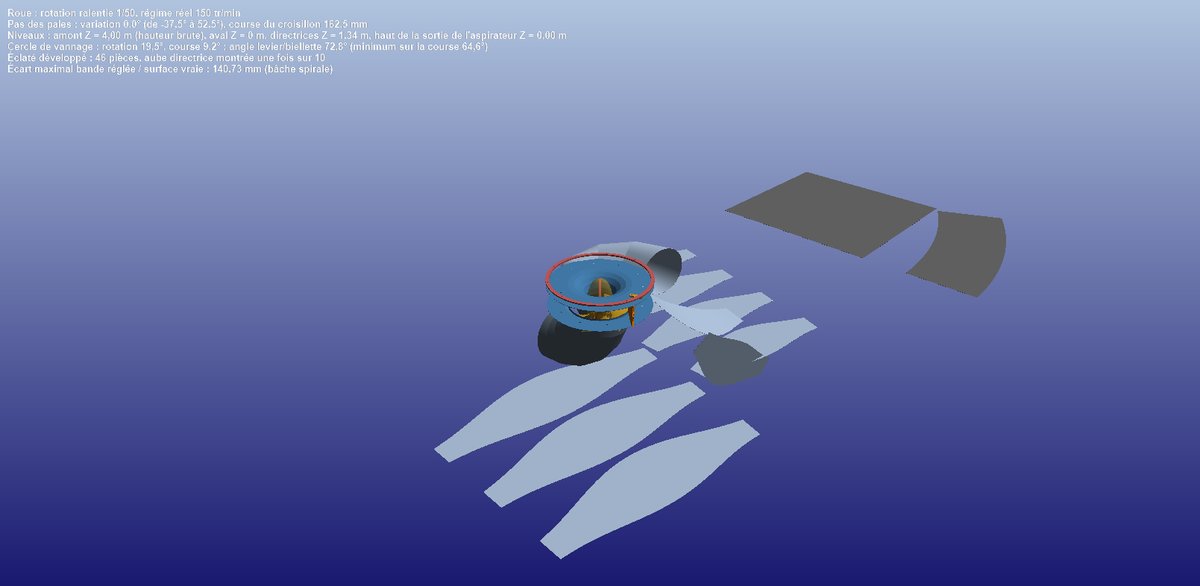
The Kit tab unfolds the structure into 46 developed sheets, with bill of materials and drawings, gate ring and pitch mechanism included.
The study files are available for download: the study centrale_12m3s_4m.hydt (to open in Hydro Turbine design, which replays the calculation) and the project centrale_12m3s_4m.hlc (the runner, to open with Heliciel).
7: For the record: the manual method
Before Hydro Turbine design, we carried out this same balance by hand. The head losses were computed in Mecaflux: an inlet cone from 3 m to 1.9 m at 30° for 8 m³/s cost 25 mm, a blade cascade deflecting by 60° several meters. The suction of the draft tube was computed with the Bernoulli application of Mecaflux between its runner outlet and the reservoir: from 2 m/s to 0.5 m/s, 1,875 Pa of suction. Then we took the runner back into Heliciel with the menu for simulating a localized downstream suction, we reran the search for the optimum speed, and we compared, in a spreadsheet, the head absorbed by the runner with the losses of the circuit over a range of flow rates: their intersection with the gross head gave the operating point. Hydro Turbine design finds this intersection with its solver and displays the balance live, but the logic is the same, and understanding it is the real know-how of turbines in conduits.
We end this tutorial here. To go further, we can go back to the design method, open the full user guide of Hydro Turbine design, or work on a more modest site with the 238 mm Kaplan micro-turbine.
 Global site map
 Mecaflux
 Tutorials Mecaflux Pro3D
 Tutorials Heliciel
 Tutorials Heliciel PRO CFD
 Mecaflux Store
 Compare software functions
 Quotes, Orders, Payment Methods
 project technical studies